What do the retina and V1 know about spatial frequencies in natural scenes?

Take a look at the picture below. Focus on how far up on the picture does the grating seem to disappear. It is different at different spatial frequencies, and traces out a curve, depending on how far away you are viewing the image. (Try zooming out or zooming in, and at some point the boundary between the visible and the invisible will match the yellow curve.)

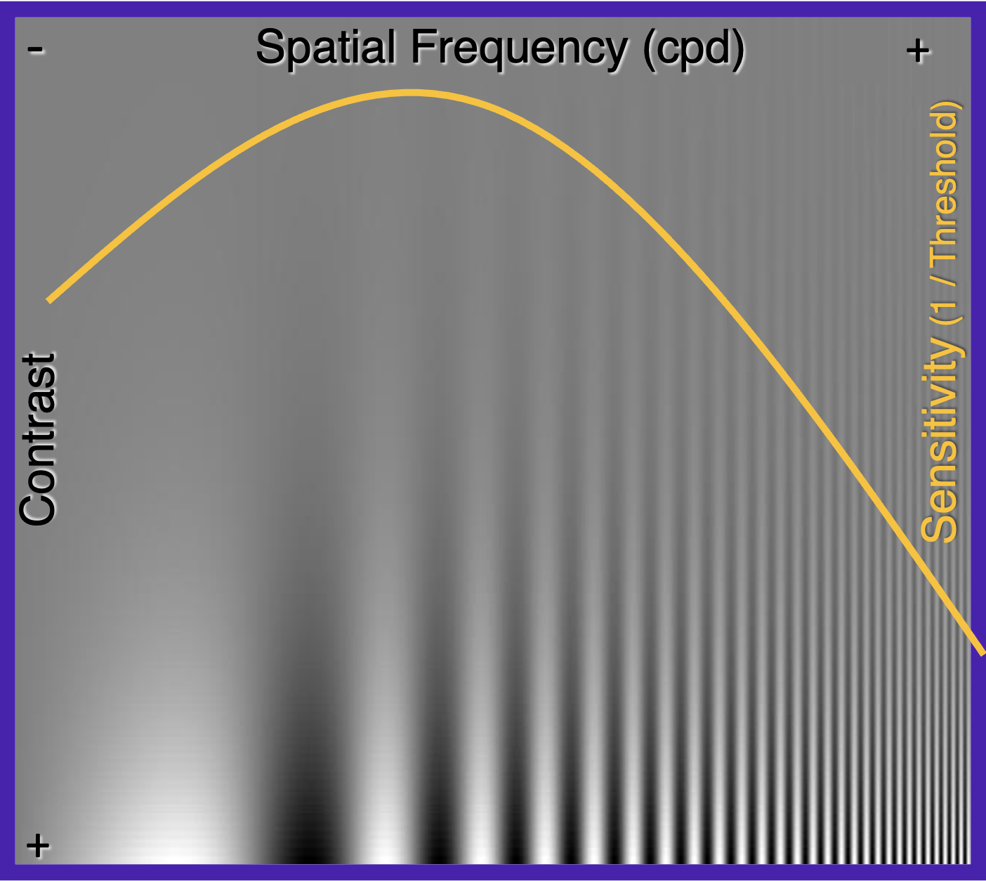
This inverted U-shaped curve, called the contrast sensitivity function (CSF), basically describes the phenomenon that our sensitivity to the middle frequency gratings is the strongest, but as we go from middle to the sides to higher or lower frequencies, our ability to detect the gratings get worse.

Sensitivity and detection threshold are concepts on two sides of a coin. Low sensitivity means that the detection threshold (the contrast above which the signal is detectable) is high. At any spatial frequency, contrast sensitivity is the inverse of contrast detection threshold.

The right half’s downward trend is somewhat expected since our photoreceptors are physically limited to have finite fidelity or a “cutoff frequency”. But the other half is more puzzling. Here, I’m going to introduce a theoretical explanation and propose a neural mechanism for the left half of the shape which is an upward trending, almost straight line.

The Retina

Atick and Redlich (1992) identified an interesting coincidence between the lower frequency range of the CSF and the spatial power spectrum calculated by Field for natural images. Think of the “power” here as a meaasure of how correlated the brightness of the pixels are locally in an image. It turns out that it is high for low frequencies and low for high frequencies, and when plotted against frequency on a log-log scale, it forms a negatively sloped straight line: \(\begin{align} R(\mathbf{f}) = 1/\mathbf{f}^2\label{eq1}\tag{1} \end{align}\) where \(\mathbf{f}\) is spatial frequency and \(R(\mathbf{f})\) is the Fourier transform, \(\int{d\mathbf{x}e^{i\mathbf{fx}}R(\mathbf{x})}\), of the autocorrelation of luminance between two points on an image: \(R(\mathbf{x}_1, \mathbf{x}_2)\). Assuming the relation between two arbitrary points anywhere in a natural scene is roughly homogeneous, this autocorrelator is then a function of only the distance between two points: \(\begin{align} R\left(\mathbf{x}_1 = (x_1,y_1), \mathbf{x}_2 = (x_2,y_2)\right) &= \langle L(\mathbf{x}_1)L(\mathbf{x}_2)\rangle \\ &= R\left(\mathbf{x} = \mathbf{x}_1 - \mathbf{x}_2\right) \label{eq2}\tag{2} \end{align}\)

Atick and Redlich noticed that the psychophysical CSF multiplied with the amplitude spectrum \(\sqrt{R(\mathbf{f})}\) makes a flat curve in the low frequency range. They went on to reason from the mechanism of the retinal ganglion cells that if we assume that all RGCs work as filters with linear kernels, meaning that the luminance outputs of the retina are \(O(\mathbf{x}_j) = \int{d\mathbf{x}_iK(\mathbf{x}_j-\mathbf{x}_i)L(\mathbf{x}_i)}\), then in frequency space the \(K(\mathbf{f})\) is a bandpass filter. Could this be what determines the shape of the psychophysical CSF?

Back then they did not have the experimental data of the retinal CSF (the actual RGC bandpass filter), so they proposed that theoretically it would be nice for the retinal CSF to have the same shape as the psychopysical CSF. Because

1) the output power spectrum of the retina (averaged over trials) would be \(\begin{align} \langle O(\mathbf{f})O^*(\mathbf{f})\rangle &= \langle(K(\mathbf{f})L(\mathbf{f}))(K(\mathbf{f})L(\mathbf{f}))^*\rangle \label{eq3}\tag{3}\\ &= \langle L(\mathbf{f})L^*(\mathbf{f})\rangle \langle K(\mathbf{f})K^*(\mathbf{f})\rangle \label{eq4}\tag{4}\\ &= R(\mathbf{f}) \left(CSF(\mathbf{f})\right)^2 \label{eq5}\tag{5} \end{align}\) which is flat, accomplishing whitening of the visual input. This can be understood as decorrelation, since \(\langle O(\mathbf{f})O^*(\mathbf{f})\rangle\) being constant in the frequency domain means that in the spatial domain it is a delta function: \(\langle O(\mathbf{x}_i)O^*(\mathbf{x}_j) \rangle \sim \delta_{ij}\). Reducing correlation is consistent with the redundancy reduction idea by Barlow, which is an efficient coding strategy;

2) they would have found a normative explanation for the upward sloping part of the psychophysical CSF.

However, as it turned out, the parvo and magno RGCs in the human and monkey retina were later found not to have such a significantly upward sloping CSF in the low frequency range but rather a quite flat one. So Atick and Redlich’s theory proved to be incorrect in attributing the whitening function to the retina. Nonetheless, their theory was useful in pointing out that the psychophysical CSF may serve the purpose of whitening visual input across spatial frequencies.

The Primary Visual Cortex (V1)

The next candidate in line to take credit for the psychophysical CSF is V1. If retina does not know whitening, then V1 probably has to. The question is how, and whether this redundancy reduction goal would be in conflict with the specific type of efficient coding strategy discussed in my previous post.

To limit the scope of analysis, we have to make a simplifying assumption (but see e.g. Skyberg et al 2022). Let’s assume that V1 processes all information across all spatial frequencies with the same speed at the same time.

Now the question is: can V1 accomplish two objectives at once:

1. Whiten the spatial power spectrum (as in Atick & Redlich)
2. Dedicate more encoding resources (Fisher Information) to the more prevalent spatial frequencies (as in Wei & Stocker)

Objective 1 means that the V1 neurons preferring low spatial frequencies should have a peak firing rate that is lower than their high-frequency preferring colleagues, while objective 2 means that the low-frequency preferring V1 neurons should encode higher-fidelity information with the small range of firing rates they are left with due to objective 1. Specifically, assuming that the amplitude spectrum (\(1/f\)) is a good proxy for the prior distribution of spatial frequency in natural scenes, then Fisher Information (FI) should be allocated according to: \(J(f) \propto 1/f^2\).

This immediately begins to seem like a demanding job for the low-frequency neurons. Now add that to the distribution of V1 neurons’ preferred spatial frequencies experimentally measured by Foster et al, similar to the lower-left histogram in figure 2 below.

Given all the objectives and constraints, designing the desired tuning profile is herculean task without the help of an algorithm. So I wrote one to find a solution for me. The optimization result is shown in figure 2, where the upper-left is the tuning profile, and the other subplots spell out the constraints and objectives that I used, consistent with what we have listed above.

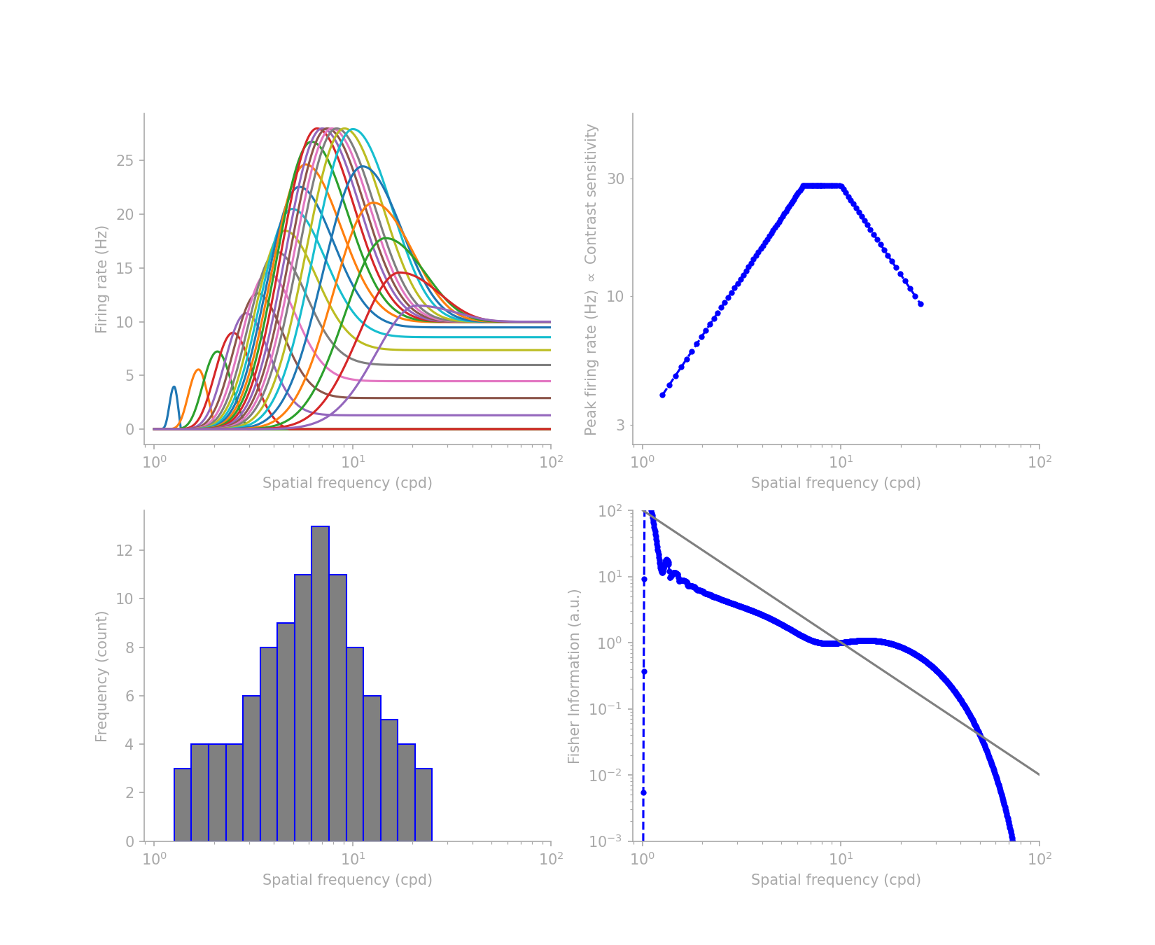
I will share in a future post the code for the gradient descent algorithm I used and how I parameterized the tuning curves, but here suffice it to say that I abused the flexibility of the Beta distribution and added parameters for the base firing rates on the left and right edges of each tuning curve.

Ignoring the FI profile beyond the cut-off frequencies, which is beyond the range in the histogram, the FI profile can come close to the target \(1/f^2\) shape, assuming Poisson noise. What the low-frequency preferring neurons lack in number, they make it up by inviting their higher-frequency preferring neighbors to extend their tuning farther into the low-frequency range. On the high-frequency extreme, though it is not the focus of this post, where low FI is needed, the neurons achieve it by increasing the base firing rate and thus decreasing the slope of the tuning curves in the high frequency direction.

This goes to show that it is still possible, although demanding, for V1 to accomplish two efficient-coding related objectives at once, even without considering temporal dynamics.

Finally, let’s come back to the initial assumption. In fact, experimentalists have demonstrated that our visual system probably processes spatial frequency information in a coarse-to-fine temporal sequence, which means that the high-frequency preferring neurons fire after the low-frequency preferring ones. This would break our initial assumption that has limited our analysis to a static one.

So it may turn out that various temporal dynamics is the key to understanding what V1 really knows about natural scenes. But that’s for another post to scratch the surface of.