What does V1 know about orientations in natural scenes?

Horace Barlow put forth the efficient coding hypothesis in 1961 which has proved to be fundamentally useful for understanding and modeling how the brain encodes sensory information. So useful, in fact, that it is now often referred to as the efficient coding theory, or the efficient coding principle instead.

The principle suggests that under strict resource constraints, our sensory system must have become near-optimal in maximally preserving sensory information given the statistics of naturally occurring stimuli. In plain words, with the limited neuronal resources we have, we must have learned (through evolution, development, or adaptation) to be efficient in allocating these neurons for processing what we typically see, hear, touch, smell, etc., in a given environment.

Let’s start with an example from vision to demonstrate how this idea is formalized, and to make the principle concrete.

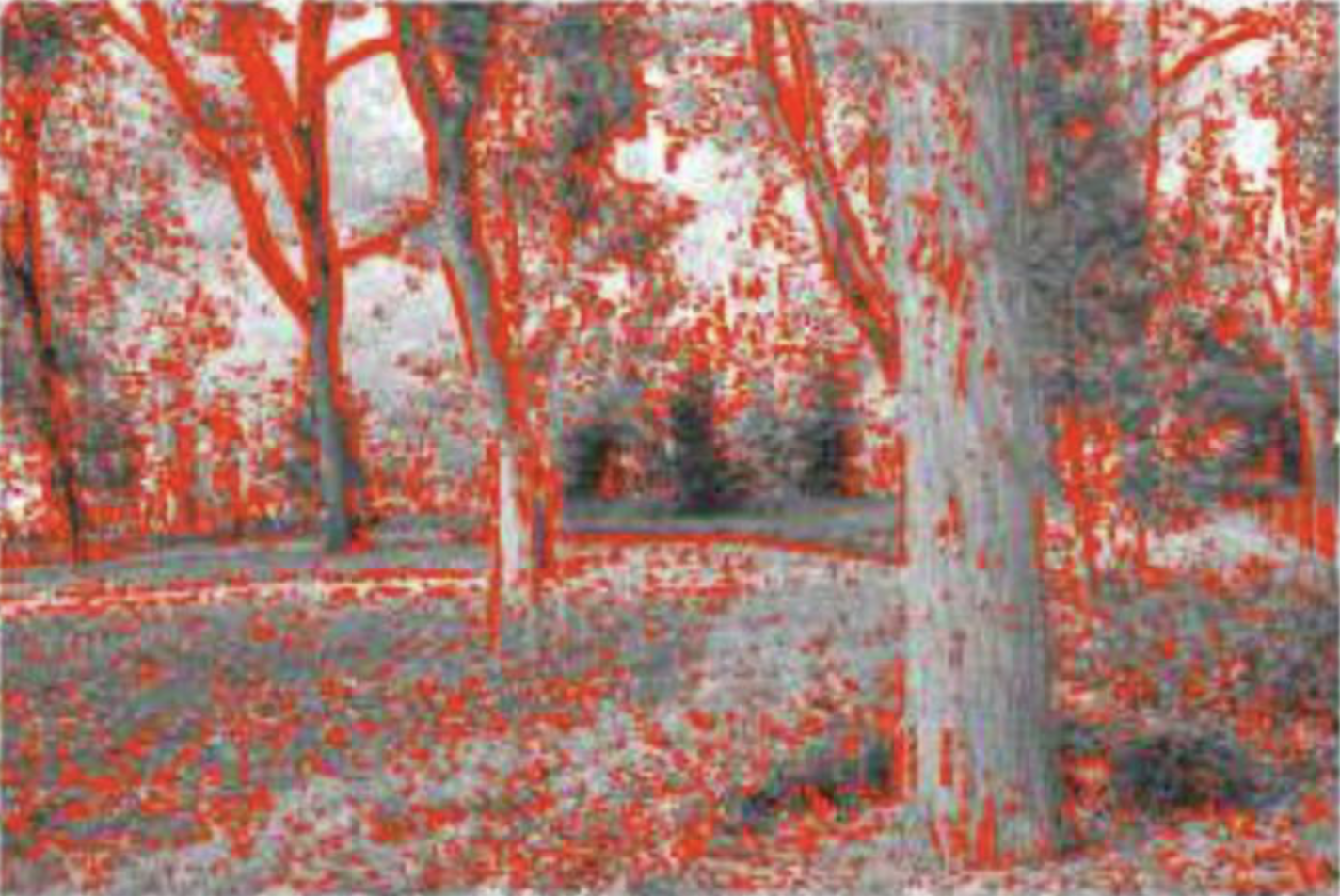
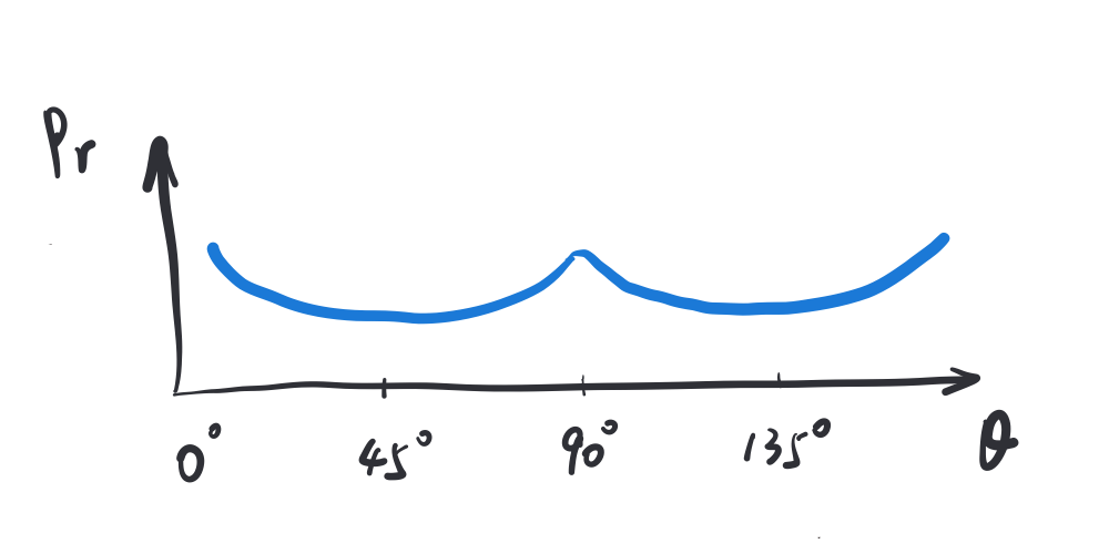
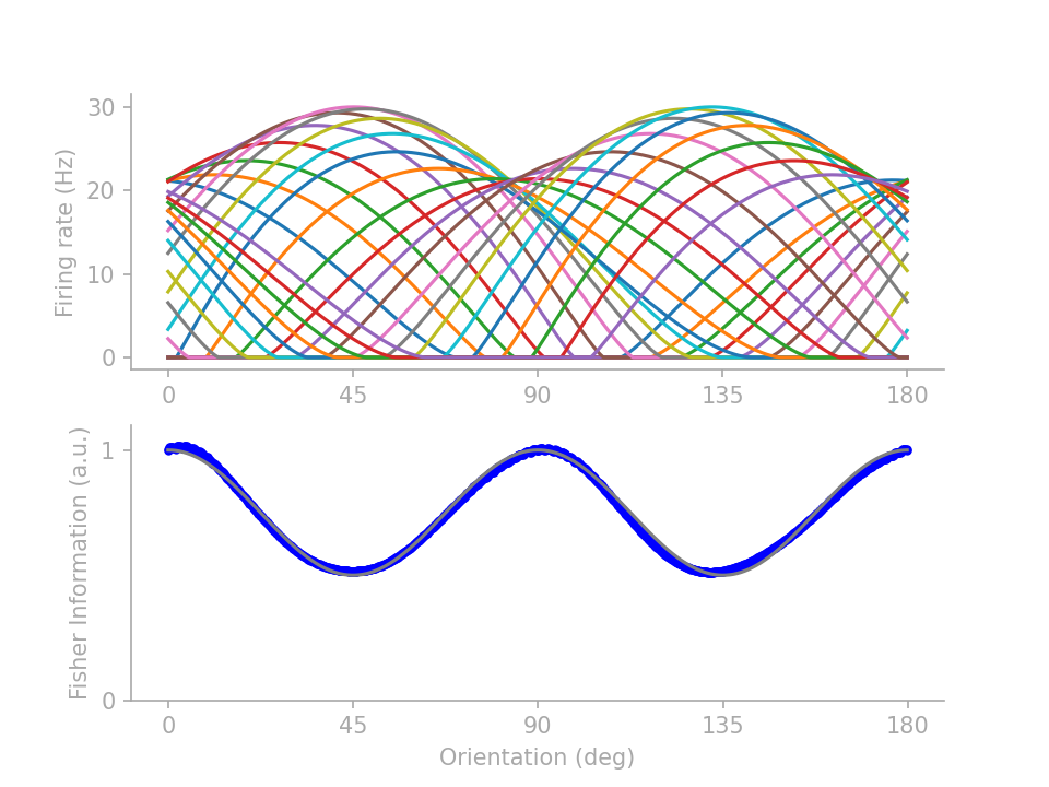
Statistically speaking, in the natural environment, the orientations of local structures in an image are not uniformly distributed. More structures are cardinal (vertical/horizontal) than oblique (45/135 deg) (see, e.g., Girschick et al).

To maximize the encoding efficiency for orientation, the visual system should arrange its tuning curves to maximize the mutual information between the orientation \(\theta\) and the neural activity \(r\) encoding orientations. Intuitively speaking, high mutual information means that by observing the neural encoding of orientation, a decoder can obtain much information about the actual orientation, and vice versa.

This mutual information quantity, written as \(I[\theta, r]\), is a function of the joint and marginal distributions of \(r\) and \(\theta\) and is closely related to the Shannon entropy of each of the two variables (since entropy is also a function of a variable’s distribution). As it turns out, \(I[\theta, r]\) can also be written in terms of the Fisher Information (see my previous post, here a function of orientation) and the distribution of orientations in the environment: \(\begin{align} I[\theta, r] &= I[f(\theta), r] = H[r] - \int{d\tilde{\theta}p(\tilde{\theta})H[r|\tilde{\theta}]}\label{eq1}\tag{1}\\ &= H[r] - \int{d\tilde{\theta}p(\tilde{\theta})H[\delta]}\label{eq2}\tag{2}\\ &= H[r] - \int{d\tilde{\theta}p(\tilde{\theta})\left(\frac{1}{2}\ln\frac{2\pi e}{J(\delta)}+D_0\right)}\label{eq3}\tag{3}\\ &= (H[r] - H[\tilde{\theta}]) + H[\tilde{\theta}] - \frac{1}{2}\int{d\tilde{\theta}p(\tilde{\theta})\ln\frac{2\pi e}{J(\tilde{\theta})}} - D_0\label{eq4}\tag{4}\\ &= H[\theta] - \frac{1}{2}\int{d\theta p(\theta)\ln\frac{2\pi e}{J(\theta)}} + C_0 - D_0\label{eq5}\tag{5}\\ &= \frac{1}{2}\ln\frac{(\int{\sqrt{J(\theta)}d\theta})^2}{2\pi e} - KL\left(p(\theta)||\frac{\sqrt{J(\theta)}}{\int{\sqrt{J(\theta)}d\theta}}\right)+ C_0 - D_0 \label{eq6}\tag{6} \end{align}\)

where:
    (i) \(g(\theta) = \tilde{\theta} = E[r|\theta]\) is the tuning function and assumed to be invertible.
    (ii) \(\delta\) in \eqref{eq3} is the additive noise (i.e., \(\delta = r - \tilde{\theta}\)) whose entropy, per Stam’s Inequality, is minimized iff \(\delta\sim\mathcal{N}(\mu,\sigma^2)\), where it also happens that \(J(\delta)=1/\sigma^2\). Thus, \(D_0\) is the entropy difference between its actual distribution and the entropy-minimizing Gaussian.
    (iii) \(C_0 = H[r] - H[\tilde{\theta}]\), where \(H(.)\) is the Shannon entropy.
    (iv) And finally, \(J(\tilde{\theta}) = J(\delta)\) since the \(p(r|\tilde{\theta})\) terms that appear in the definition of \(J(\tilde{\theta})\) are really just \(p(\delta)\).

The entire derivation was provided in Wei & Stocker’s 2016 paper. Note that \(C_0\) and \(D_0\) do not matter asymptotically under vanishing Gaussian noise. And for the purpose of this post, let’s assume the Gaussianity of and size of noise is near that regime. Thus to maximize the whole expression is to minimize the KL term, which is achieved when \(p(\theta)\propto\sqrt{J(\theta)}\). In other words, orientation encoding is most efficient when the orientation sensitive neurons’ tuning profile achieves a Fisher Information profile that matches the squared distribution of orientations in the environment!

One intuitive way to form such a tuning profile is simply to have more neurons tuned for (or sensitive to, or in charge of processing) cardinal orientations and fewer neurons for oblique orientations.

Useful and intuitive as it is, the fact that this result boils down to the principle of “allocating more neurons for the more frequently encountered stimulus feature values” is a bit too reductive, but if you are new to efficient coding, this simple intuition would suffice as your main takeaway.

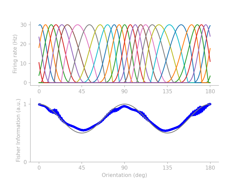
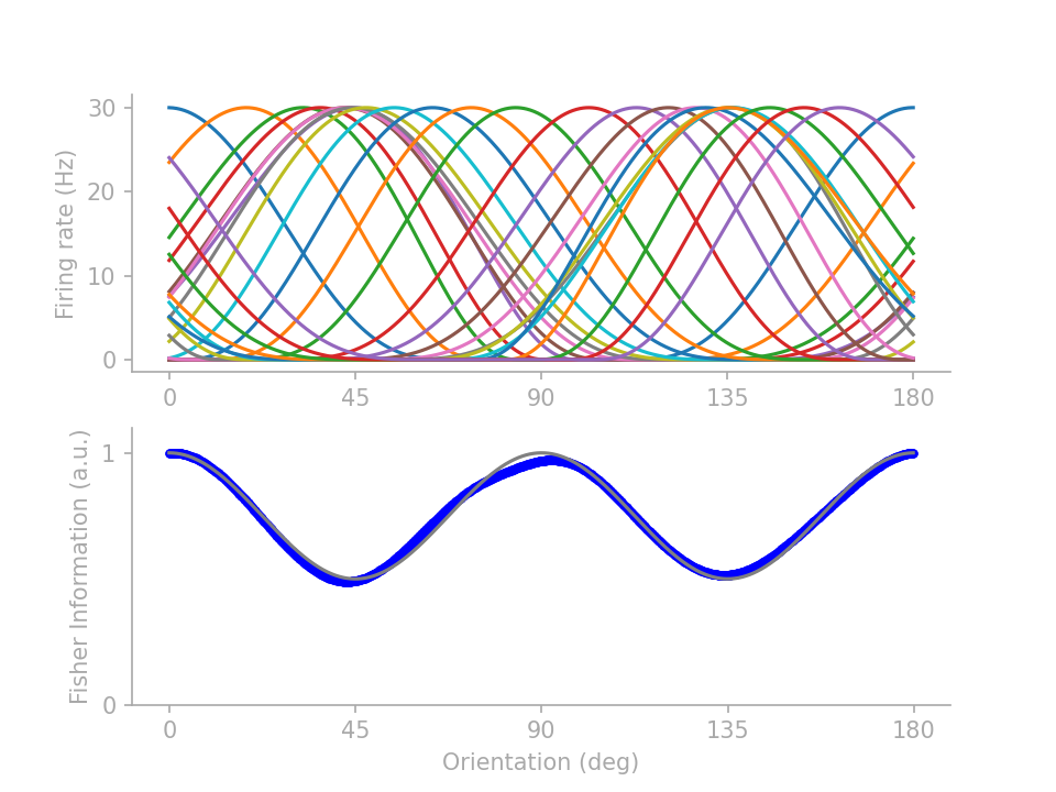
If you are reading on, here are two lines of fine prints under the simple intuition. First of all, unintuitive tuning profiles abound for achieving the same FI profile. By parameterizing the tuning curves and training the parameters to minimize a mean-squared-error loss between the target and actual FI profiles, I can generate several distinctive tuning profiles all satisfying the same FI target profile. From those I picked 3 representative profiles to showcase the intricacy that belies the simple intuition of “more neurons for the more frequent orientations”.

In figure 2 below, profiles 1 and 2 (identified in Wei & Stocker 2015) show that \(J(\theta)\) is not determined by the number of neurons preferring \(\theta\) but how many neurons have tuning curves crossing \(\theta\). Profile 3 demonstrates that tuning curve height does not necessarily drive up FI, although note that here I assume “multiplicative” Gaussian noise (Gaussian variance scales linearly with the expected firing rate), as opposed to Gaussian noise with a fixed variance.

The second point I am going make will be of no consequence under the natural image statistics that we typically care about, but may provoke some thoughts about what may happen in a strange world. Going back to the derivation from \(1\) to \(6\), we have glossed over an important assumption that in fact enabled us to link efficient orientation encoding and the fundemental principle of preserving maximal information content from an image in the first place.

In \eqref{eq1} it may have appeared that \(H[r\\|\theta]\) is only a function of \(\theta\) but not other visual features. But as we know, a V1 neuron is selective for both orientation and other features such as spatial frequency. This means that the firing rate \(r\) simultaneously or jointly encodes information about both \(\theta\) and frequency \(f\).

To see why this could matter in pathological cases, we rewrite \eqref{eq1} as:

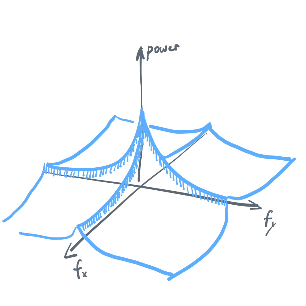
\[\begin{align} I[\theta, r] &= H[r] - \int{\left( \int{H[r|\theta, f]p(f|\theta)df}\right)p(\theta)d\theta}\label{eq7}\tag{7} \end{align}\]

Note that \eqref{eq7} is only equal to \eqref{eq1} when we assume that either \(H[r\\|\theta,f]\) is independent of \(f\) or \(p(f\\|\theta)\) is independent of \(\theta\), the latter of which turns out in fact to be true. (As a side note, \(p(\theta\\|f)\) is also independent of \(f\). See the following joint power spectrum in figure 3.)

But what would happen to the efficient coding solution for \(J(\theta)\) if, hypothetically, both are untrue? For example, \(H[r\\|\theta,f]\) could depend on \(f\) for reasons such as redundancy reduction, and once we find a world where \(p(f\\|\theta)\) somehow is drastically different around some orientation, the efficient coding strategy for \(\theta\) will no longer have a simple dependence on \(p(\theta)\). Such a strange world is certainly not impossible to find.