Noise and two simplified forms of Fisher Information

Fisher information (FI) is a measure of information (though not a strict information quantity) and is commonly used in neuroscience. But when I was new to the concept, it seemed hard to grasp because of its connection with many other concepts in neuroscience. This post is a quick introduction to some frequently used conclusions and remarks about FI in neuroscience. I assume that you already understand what neural tuning curves and firing rate noise are.

At the end of the post I provide derivations for 2 basic results: 1) \(J(\theta) = f’(\theta)\) if firing rate noise is Gaussian and 2) \(J(\theta) = f’(\theta)^2 / f(\theta)\) when Poisson firing is assumed. This can serve as a primer to understanding the use of FI in Kriegeskorte and Wei’s 2021 review paper.

The original formulation of Fisher Information

In plain language and speaking generally, Fisher Information (FI) quantifies the amount of “information” an observable random variable \(r\) carreis about its parameter \(\theta\). The formal way that this quantity came to be defined by Ronald Fisher was:

\[\begin{align} J(\theta) = Var(l'(r|\theta)) = \int{\left(-\frac{d}{d\theta}\log p(r|\theta)\right)^2p(r|\theta)dr} \label{eq1}\tag{1} \end{align}\]

where \(l(r|\theta)\) is the log-likelihood of \(\theta\), \(\log p(r|\theta)\), and the second equality is based on the equivalence between \(Var(.)\) and \(E(.^2) - E^2(.)\).

The definition introduced in the paper is yet another equivalent form:

\[\begin{align} J(\theta) = \int{-\frac{d^2}{d\theta}\log p(r|\theta)p(r|\theta)dr} \label{eq2}\tag{2} \end{align}\]

which can be verified noticing: \(-(\log x)’’ = -(1/x)’ = 1/x^2 = ((\log x)’)^2\).

Now personally, I think this form in \eqref{eq2} gives a more intuitive way of understanding FI, since it can be seen as the expectation of the second derivative of the negative log-likelihood (NLL) function. The maximum-likelihood estimator (MLE) for \(\theta\) given \(r\) is obtained when the first derivative of the NLL is zero, where the NLL has a local trough (local peak for the log-likelihood function). Looking further at the second derivative tells us how sharp the trough is, and hence quantifies the “precision” of the MLE.

Fisher Information in neuroscience

In neuroscience the situation where we care about this information is when \(r\) is the internal representation or encoding of the stimulus \(\theta\) and we want to measure how much information a reading of this internal representation (typically in the form of neural firing rates) conveys about the stimulus \(\theta\) that caused this much neural activity in the first place.

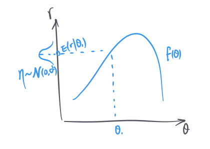
\(r\) can be a vector of activities of multiple neurons, but for simplicity let’s assume it is just one neuron. The neuron reacts to different stimulus values differently following a tuning function \(f(\theta)\), and on top of that, it is also noisy. Generatively speaking, given a stimulus value \(\theta_0\), the neuron’s activity \(r\) is \(f(\theta_0) + \eta\) where \(\eta\) can be modeled as a stimulus-independent Gaussian noise. In some cases, it can be more accurate to model the noise as stimulus-dependent Gaussian, or simply to model \(r\) as following a Poisson process with \(f(\theta_0)\) as the mean.

To visualize the tuning transform and the noise in the same picture:

Two simplified forms of FI

So far the basic definitions may have appeared complicated, especially the definition of FI. But as the authors mention in the paper, specific noise assumptions actually simplify the expression of FI.

1) If we assume stimulus-independent Gaussian noise with variance 1, then FI is simply: \(\begin{align} J(\theta) = f'(\theta)^2, \label{eq3}\tag{3} \end{align}\)      where \(f(\theta)\) is the tuning function.

2) If we assume Poisson spiking, then FI can be shown to have the following form instead: \(\begin{align} J(\theta) = \frac{f'(\theta)^2}{f(\theta)} \label{eq4}\tag{4} \end{align}\) Here I provide the proofs. Hopefully with the background introduction on what the tuning \(f(\theta)\) is and where the noise comes in, these become easy to understand.

Proof for \eqref{eq3}: When \(p(r|\theta)\) is Gaussian: \(\begin{align} \log p(r|\theta) &= -\frac{(r-f(\theta))^2}{2\sigma^2} + const. \label{eq5}\tag{5}\\ J(\theta) &= -E_{r|\theta}[\frac{d^2}{d\theta^2}\log p(r|\theta)] \label{eq6}\tag{6}\\ &= -E_{r|\theta}[\frac{d^2}{d\theta^2}(\frac{rf(\theta)}{\sigma^2}-\frac{f(\theta)^2}{2\sigma^2})] \label{eq7}\tag{7}\\ &= -E_{r|\theta}[\frac{rf''(\theta)}{\sigma^2}-(\frac{2f(\theta)f'(\theta)}{2\sigma^2})'] \label{eq8}\tag{8}\\ &= -E_{r|\theta}[\frac{rf''(\theta)}{\sigma^2}-\frac{f'(\theta)^2}{\sigma^2}-\frac{f(\theta)f''(\theta)}{\sigma^2}] \label{eq9}\tag{9}\\ &= -E[-\frac{1}{\sigma^2}f'(\theta)^2] \label{eq10}\tag{10}\\ J(\theta) &= f'(\theta)^2 \label{eq11}\tag{11} \end{align}\)

\eqref{eq9} to \eqref{eq10} is because \(E_{r|\theta}(r) = f(\theta)\), and \eqref{eq10} to \eqref{eq11} is assuming \(\sigma = 1\).

Proof for \eqref{eq4} follows the same procedure. If \(p(r|\theta)\) is Poisson: \(\begin{align} \log p(r|\theta) &= \log \frac{f(\theta)^re^{-f(\theta)}}{r!} = r\log f(\theta) - f(\theta) - \log r! \label{eq12}\tag{12}\\ J(\theta) &= -E_{r|\theta}[r(\frac{f'(\theta)}{f(\theta)})'-f''(\theta)] \label{eq13}\tag{13}\\ &= -E_{r|\theta}[r \frac{f''(\theta)f(\theta)-f'(\theta)^2}{f(\theta)^2}-f''(\theta)] \label{eq14}\tag{14}\\ &= -[f''(\theta)-\frac{f'(\theta)^2}{f(\theta)}-f''(\theta)] \label{eq15}\tag{15}\\ J(\theta) &= \frac{f'(\theta)^2}{f(\theta)} \label{eq16}\tag{16} \end{align}\)

Now so far we have been assuming that \(r\) is a scalar, namely that only one neuron encodes \(\theta\). When multiple neurons encode the parameter together, as long as the neurons have independent noise, the FI is just the sum of the FI for individual neurons.

Finally, if \(\theta\) itself is multidimensional, then \(J(\theta)\) becomes a matrix, e.g., \( \mathbf{J}(\theta_1, \theta_2) \) where \(\begin{align} \mathbf{J}_{11} &= J(\theta_1, \theta_2=\theta_2) \\ \mathbf{J}_{22} &= J(\theta_1=\theta_1, \theta_2) \\ \mathbf{J}_{12} &= \mathbf{J}_{21} = J(\theta_1, \theta_2) \end{align}\)